Cross-Dataset Statistical Analysis

METASPACE Pro

Only available for METASPACE Pro users.

What it is

Cross-Dataset Statistical Analysis lets you test which ions differ significantly between experimental conditions, pooling regions from several datasets within a project into one statistical comparison. You build an Experiment: a named collection of regions drawn from your project's datasets, each tagged with the sample metadata that describes your experimental design (which condition it belongs to, which biological sample it came from, and so on). METASPACE then fits a moderated statistical model, based on the limma methodology from genomics, to every annotated ion and reports which ones change significantly between conditions.

A region can be a manually drawn ROI, an automatically generated segmentation cluster, or a whole dataset treated as a single sample. You choose the region source independently for each dataset you add, so an experiment can mix, for example, hand-drawn tumor ROIs from one dataset with whole-dataset samples from another, as long as the underlying comparison makes biological sense.

The statistical engine behind this feature was chosen specifically because METASPACE experiments rarely have more than a handful of biological replicates per condition. Ordinary per-ion tests (a t-test or a Wilcoxon test run independently on each ion) are unreliable at that sample size: individual variance estimates are too noisy to trust, and Wilcoxon-style rank tests can't even reach a significant p-value with only 2-3 samples per group, however strong the real effect is. The interpretation guide explains how the underlying model works around this; this page focuses on how to set up and run an experiment.

When to use it

• You have the same or comparable tissue sampled under different conditions (treated vs. control, disease vs. healthy, different timepoints), and each condition lives in its own dataset or datasets.
• Your samples have both biological replicates (different animals, patients, or tissue sections) and, optionally, technical replicates (repeated acquisitions of the same physical sample), and you need those modeled correctly rather than treated as identical independent evidence.
• You only have a handful of replicates per condition (as few as 3) and need a test with enough statistical power to call real differences significant despite that.
• You want to compare more than two conditions at once (e.g., control / early / late) and see both an overall "does this ion change at all across conditions" result and the specific pairwise differences behind it.
• You want to reuse regions you've already defined, such as ROIs from ROI Selection or clusters from Spatial Segmentation, as the sampling units for a cross-dataset comparison, instead of defining new regions from scratch.

How to use it

Setting up an experiment involves more decisions than most METASPACE features, because you're describing your experimental design to the statistical model, not just picking a dataset to view. The steps below walk through the decisions in order; the video covers the same flow end to end.

1. Create the experiment

From a project, start a new experiment and give it a name and, optionally, a description. This is also where you pick the match mode, which controls how regions from different datasets are paired up later:

• NAME automatically matches regions that share the same label across datasets: an ROI called Tumor in every dataset lines up automatically. This is the fastest option when your datasets already use consistent region naming.
• MANUAL skips automatic matching and lets you map regions between datasets yourself. Use this when region names differ across datasets, or when there's no natural one-to-one correspondence between them.

2. Add datasets and choose a region source

Add every dataset from the project that contributes samples to the experiment. An experiment stays within a single project, so pick a project whose datasets already cover the comparison you want to run. For each dataset, choose its region source:

• ROI — uses regions you drew with ROI Selection.
• Segmentation — uses clusters from a completed Spatial Segmentation run.
• Whole dataset — treats the entire dataset as a single region, i.e. one sample.

If a dataset uses ROIs and another dataset in the experiment already has ROIs defined, you can copy the ROI set across so you don't have to redraw the same boundaries by hand.

3. Describe your samples

For every region, fill in the metadata that defines your experimental design:

• Condition — the experimental group being compared (e.g. control, treated). This is the variable the statistical test looks for differences across, and it's the single most important field: get this wrong and the whole comparison is wrong.
• Biological replicate ID — identifies which biological sample (animal, patient, tissue block) a region actually came from. This is what lets the model recognize a paired design: the same biological replicate ID appearing under more than one condition tells the model those measurements are linked, not independent.
• Sample ID — a human-readable identifier for the physical sample. METASPACE infers a reasonable default from the dataset name and region label, but you can override it.
• Technical replicate ID (optional) — marks repeated acquisitions of the same physical sample. Regions sharing a technical replicate group are averaged together into one value before the statistical test runs, so repeat scans strengthen your estimate of that sample rather than being miscounted as extra independent replicates.
• Batch ID (optional) — records which acquisition batch or run a sample belongs to. This is for your own tracking and for spotting batch-driven patterns during quality control; it is not currently used as a statistical covariate in the model.

Metadata is entered per dataset, with bulk-assignment tools available so you don't have to repeat yourself region by region when many regions share the same condition or replicate.

4. Assign label groups

Label groups let you run more than one independent comparison inside the same experiment. Every region belongs to exactly one label group, and the statistical test (including which conditions are compared and any design warnings) is computed separately per label group. Use this when, for example, your experiment spans more than one tissue type, cell population, or anatomical structure, and you don't want those pooled into a single comparison. If you have a single, uniform comparison, everything can stay in one label group.

5. Review the analysis preview and warnings

Before running anything, METASPACE shows an analysis preview summarizing, per label group, which comparisons your current metadata will produce: which condition pairs, or an overall omnibus comparison when a label group has three or more conditions. This is the point to catch metadata mistakes, such as a condition typo that splits one group into two, or a region assigned to the wrong label group.

If a label group's design can't support a meaningful comparison yet (for instance, only one condition is present, or a condition has only a single biological replicate), METASPACE flags it inline rather than letting you discover it after the run finishes.

6. Run the experiment

Once the design looks right, run the experiment. Preparing the data (extracting and aggregating intensities across every region and ion) can take a while for large experiments, so METASPACE emails you when it's ready rather than requiring you to keep the tab open.

What results look like

Once preparation finishes, you land on a dedicated results page organized as three stages you move through in order:

1. Sample QC — signal quality and outlier detection per sample, with the option to exclude a sample and re-run.
2. Explore — annotation-level filtering (FDR, database, adduct) and per-sample ion coverage, controlling which ions are eligible for the statistical test.
3. Results — the statistical output itself: a sortable, filterable results table, a volcano plot, and a per-ion intensity strip plot, with export to CSV.

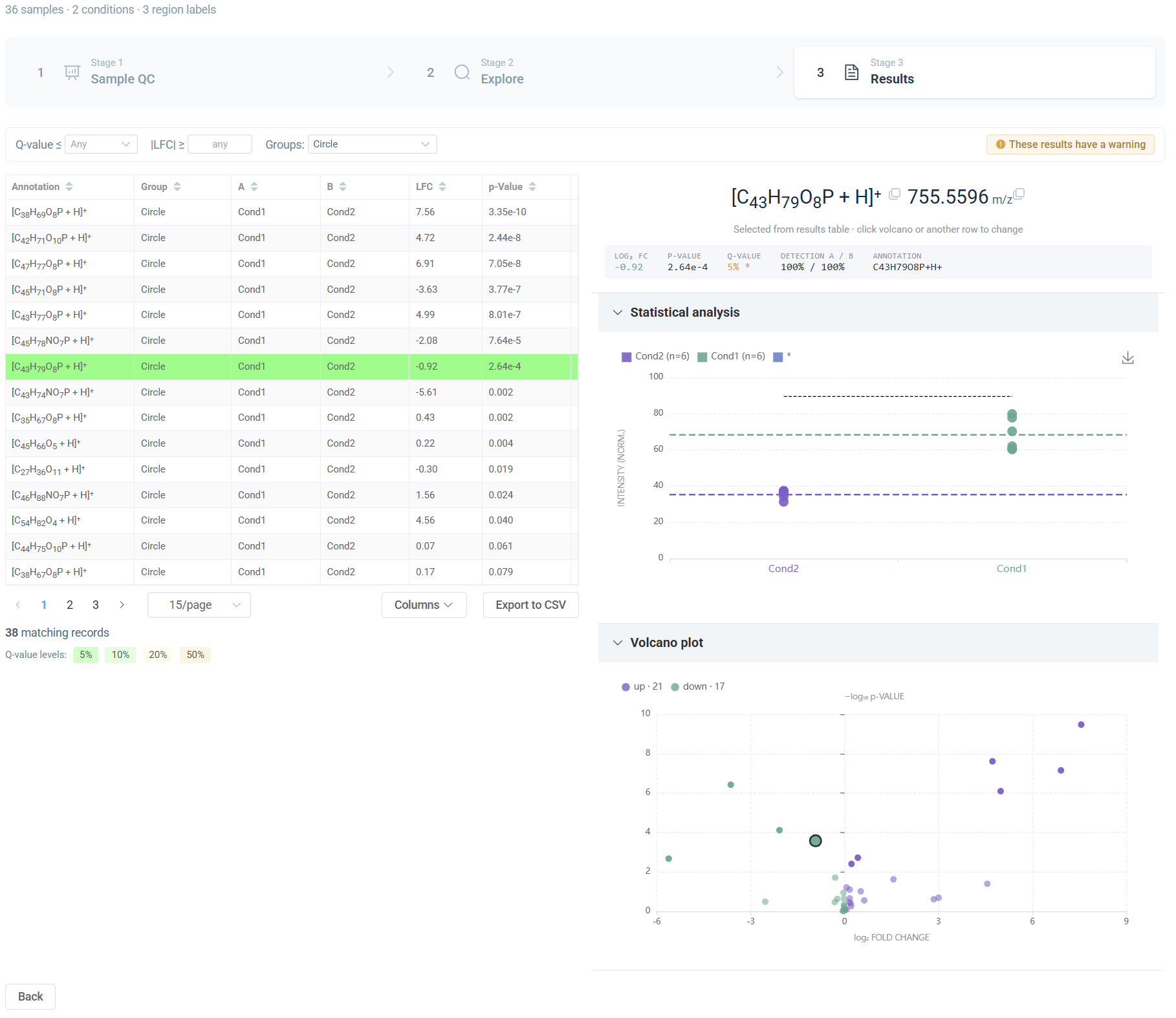Results stage showing the results table, volcano plot, and intensity strip plot for a two-condition comparison.

For a full walkthrough of each stage and how to interpret what you see, including why limma is used, what the design warnings mean, and how to read an omnibus result alongside its pairwise contrasts, see the interpretation guide.