Understanding cross-dataset statistical results

METASPACE Pro

Only available for METASPACE Pro users.

How it works

Why not a simple t-test or Wilcoxon test

METASPACE experiments typically have very few biological replicates per condition, often just 3. At that sample size, the two most common statistical approaches break down:

• A t-test per ion trusts each ion's own variance estimate on its own. With only 3 replicates, that estimate is unreliable: some ions look "significant" purely by chance, while others with a real, strong effect look non-significant simply because their particular 3 samples happened to be noisy.
• A Wilcoxon rank-sum test runs into a harder floor: with 3 samples per group, there aren't enough possible orderings of the data for the test to ever reach a small p-value, no matter how large the true difference is. It also has no way to represent the replicate structure described below: it treats every sample as independent.

Borrowing strength across ions

limma addresses the small-sample problem with empirical Bayes moderation. Rather than trusting each ion's own noisy variance estimate in isolation, limma looks at the spread of variance estimates across all ions in the comparison and uses that shared information to stabilize each individual one. Every ion's variance gets pulled toward a common, more reliable estimate, which makes the significance test far more robust when sample sizes are small. This is the step that lets METASPACE call real, meaningful differences significant with as few as 3 replicates per condition, something a plain t-test or Wilcoxon test cannot do reliably at that size.

That shared variance estimate, the prior, is deliberately not built from every ion in every region. Pooling all ions from unrelated regions together would mix in ions with genuinely different biology, inflating the variance estimate and making real effects harder to detect. Instead, METASPACE estimates the prior from a curated set of ions specific to the comparison being made: those with consistently high intensity and low noise, which are the ions whose variance is actually informative about the "typical" spread you'd expect from measurement noise alone. Every ion is still tested, including lower-intensity, noisier ones, but only the well-behaved ions inform what "normal" variance looks like.

Respecting the replicate structure

Your samples can carry two levels of replication: biological replicates (different animals, patients, or tissue sections; genuinely independent evidence) and technical replicates (repeated acquisitions of the same physical sample; not independent, since they come from the same underlying biology). limma's duplicateCorrelation step explicitly estimates how correlated repeated measurements from the same biological sample are, and folds that correlation into the statistical model. Without this step, technical replicates would be counted as if they were extra independent biological evidence, making the test overconfident and inflating the number of false positives.

One comparison, or several at once

When a label group has exactly two conditions, METASPACE reports one result per ion: the difference between those two conditions. When a label group has three or more conditions, it reports two kinds of results for every ion:

• An omnibus result — a single test answering "does this ion differ across any of the conditions?", without saying which ones.
• A pairwise result for every condition pair — the same kind of result as the two-condition case, but computed for each pair independently.

Both are computed from the same underlying model fit, so they're consistent with each other: an ion with a strong pairwise difference between two conditions will generally also show up with a low omnibus p-value.

What's precomputed vs. computed on demand

The expensive parts of this pipeline, estimating the replicate correlation and the variance prior, are computed once, when you run the experiment, and cached. Browsing the results afterward (switching between contrasts, filtering by Q-value or fold change, paging through the table) doesn't repeat that work; it's reading from the precomputed statistics, which is why the results page stays responsive even though the underlying model fit is nontrivial. Changing the experiment's design, such as adding a dataset, editing metadata, or excluding a sample, does require re-running, since it changes what the model is fit to.

Where to find it

Once an experiment finishes preparing, you're taken to its results page, organized as three stages you move through in sequence: Sample QC, Explore, and Results. You can move back to an earlier stage at any time, for example to exclude a sample you spotted as an outlier while looking at the results.

How to read it

Sample QC stage

This stage is about the raw data quality of each sample, before any statistics are computed:

• TIC (total ion current) per sample — flags samples with unusually low or high overall signal.
• Detection rate per sample — the fraction of ions detected at all in that sample, plotted against a reference line; a sample far below the others, or below the line, may have failed during acquisition or preparation.
• CV (coefficient of variation) — spread of intensities within a sample; unusually high CV can indicate a noisy or heterogeneous sample.
• PCA scatter — a 2D projection of samples based on their overall ion intensity profile. Samples that cluster tightly with others from the same condition are behaving as expected; a sample that lands far from its condition's cluster is worth a closer look before trusting the downstream statistics.

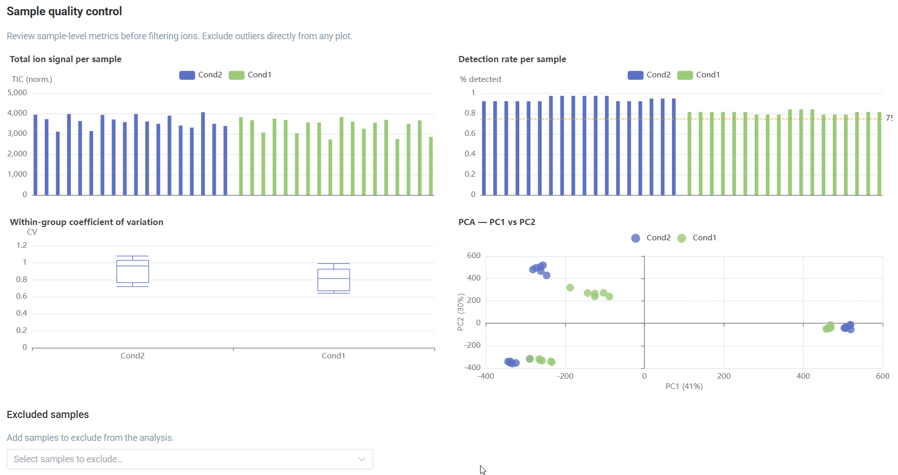TIC, detection rate, CV, and PCA scatter for a set of samples, with one sample standing apart from its condition's cluster.

You can exclude a sample from this stage using the exclude-samples list and re-run the analysis without it, useful once you've identified a clear outlier or a technical failure.

Explore stage

This stage controls which ions are eligible for the statistical test, using the same kind of annotation-level filters you'd use anywhere else in METASPACE: FDR threshold, database, adduct, and a minimum per-ion detection rate across samples. The filter-chain view shows how many ions survive each filter in sequence, and the coverage view shows per-sample ion counts after filtering.

Don't confuse this with the Q-value in the Results stage

The FDR filter here is METASPACE's annotation confidence threshold: it decides which ions are trustworthy enough to test at all. The Q-value you'll see in the Results stage is a completely different number: the statistical false discovery rate for the differential test itself, i.e. how likely a given ion's reported difference between conditions is to be a false positive. An ion can pass a strict annotation FDR and still have a high (non-significant) statistical Q-value, or vice versa. Tightening the annotation FDR filter here does not make your statistical results more significant; it only changes which ions were tested in the first place.

Results stage

This is where the statistical output lives:

• Results table — one row per ion per comparison. The Annotation column shows the ion's formula and adduct together, followed by the label Group, the condition pair being compared (columns A/B, or omnibus, with no condition pair), LFC, p-value, per-condition detection rate, and Q-value (the BH-adjusted FDR; this is the number to filter on for significance), colour-coded into the same 5%/10%/20% bins used for annotation FDR elsewhere in METASPACE. The Columns button lets you show or hide fields.
• Volcano plot — every ion plotted by log₂ fold change (x-axis) against −log₁₀(p-value) (y-axis), colored by the direction of change, with the legend totalling how many ions are up- and down-regulated at the current filters. Ions in the upper corners combine a large effect size with strong statistical support and are the most interesting first look.
• Intensity strip plot — selecting a row in the table or a point in the volcano plot opens a details panel for that ion, with its LFC, p-value, Q-value, and detection rate, and a strip plot of the actual per-sample intensity values grouped by condition. Dashed lines mark each condition's mean, and a bracket above the plot flags whether the comparison is significant. This is the ground-truth check: a low Q-value tells you a difference is statistically supported, but only looking at the individual points tells you whether it's a clean, consistent shift or a couple of samples dragging the mean around. Always look before drawing a conclusion from the table alone.
• Filter bar — restrict the table by maximum Q-value, minimum absolute LFC, and label group. When a label group has three or more conditions, a contrast selector lets you switch between viewing all pairwise comparisons, the omnibus result only, or one specific pair.
• CSV export — exports every row currently matching your filters (not just the current page), for downstream analysis outside METASPACE.
• Warnings — when a label group's design triggered one of the caveats below, a These results have a warning button appears above the table; open it for a plain-English explanation of which warning applies.

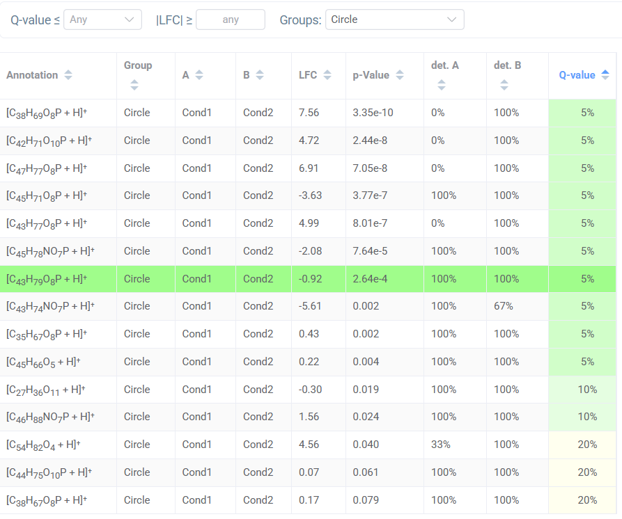Results table with LFC, p-value, and Q-value columns for a two-condition comparison.

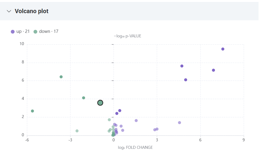Volcano plot with a cluster of ions in the upper-right corner combining a large fold change with strong statistical support.

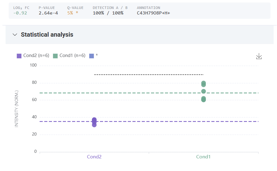Intensity strip plot for a single ion, showing per-sample values grouped by condition.

Reading omnibus and pairwise results together: with three or more conditions, start from the omnibus result (or the "all pairs" view) to find ions that change somewhere in your design, then switch to the pairwise contrasts to see exactly which condition pair is driving that change. An ion can have a significant omnibus result driven by just one condition standing apart from the rest, with no individual pair reaching significance on its own if the effect is spread thin across several comparisons. The two views answer different questions, and both are worth checking.

Common patterns and pitfalls

• Partial pairing warning — some, but not all, of your biological replicate IDs appear under every condition. limma still runs, but it can lean less on the paired structure of your design for the replicates that aren't matched across conditions.
• Unbalanced sample sizes warning — your conditions don't have equal numbers of replicates. This isn't a problem for limma by itself, but it's worth checking nA/nB in the results table alongside the Q-value, since a condition with very few samples contributes a weaker estimate.
• Partial technical replicates warning — some samples in the comparison have technical replicates and others don't. Samples with technical replicates are averaged into one value before testing; samples without them are used as-is. This is expected when your acquisition protocol wasn't uniform across samples, but worth confirming it matches what you intended.
• Multiple regions aggregated warning — more than one region shared the same biological replicate ID and condition, so METASPACE automatically averaged them into a single value before testing. This means a "replicate" in your results corresponds to a biological sample, not necessarily a single region: if you assigned two ROIs from the same tissue section to the same biological replicate ID, they were combined, not treated as two replicates.
• Single-replicate warning — a condition has only one biological replicate. The model has no within-condition variance to estimate for that condition from the data alone, so its result leans almost entirely on the borrowed (empirical Bayes) variance estimate. Treat results involving a single-replicate condition with extra caution, and add more replicates if you can.
• Experiment-wide fallback warning — no individual label group had enough data to support its own comparison, so METASPACE pooled every region across all label groups into one comparison so it could still return a result. Check whether your label group assignments were intended to be that broad.
• A tight annotation FDR filter didn't change the statistical results as much as expected — see the callout above: the Explore-stage filter and the Results-stage Q-value measure different things. Loosen or tighten the annotation filter to change which ions are tested, and use the Q-value filter to change which results you're looking at.
• A low Q-value with a messy strip plot — moderation stabilizes variance estimates, but it can't manufacture information that isn't in your data. With only a handful of replicates, one biological outlier can still meaningfully shift a result. Always check the intensity strip plot for the ions you plan to act on, not just the table.

References

• Ritchie, M. E., Phipson, B., Wu, D., Hu, Y., Law, C. W., Shi, W., & Smyth, G. K. (2015). limma powers differential expression analyses for RNA-sequencing and microarray studies. Nucleic Acids Research, 43(7), e47. https://doi.org/10.1093/nar/gkv007
• Smyth, G. K. (2004). Linear Models and Empirical Bayes Methods for Assessing Differential Expression in Microarray Experiments. Statistical Applications in Genetics and Molecular Biology, 3(1). https://doi.org/10.2202/1544-6115.1027